Appendix C: Spectral analysis

1 Introduction

Measurements of the sea-surface elevation are almost always obtained with an electrical current in some instrument. This analogue signal can be transformed into an estimate of the variance density spectrum of the waves, using analogue systems, such as electronic circuits or optical equipment. However, with today’s small and fast computers the analogue signal can also be transformed into a digital signal for a subsequent numerical analysis.

The most common and simplest measurement in this respect is a record of the sea-surface elevation at one location as a function of time (i.e., a one-dimensional record). Records like these are produced by instruments such as a heave buoy, a wave pole or a low-altitude altimeter. These can be analysed with a one-dimensional Fourier transform.⁹ Other types of measurements generate multivariate signals (i.e., several, simultaneously obtained, time records), e.g., the two slope signals of a pitch-and-roll buoy. Such signals require a cross-spectral analysis. Two-dimensional images, e.g., from a surface-contouring radar, require a two-dimensional Fourier transform and moving images (e.g., those produced by a ship’s radar) require a threedimensional Fourier transform.

The estimation of the wave spectrum from such a measurement can be based on two numerical approaches. In the first approach the auto-covariance function of the surface elevation is computed and then Fourier-transformed. The second approach is to Fourier-transform directly the wave record itself. This is the preferred technique today. It is usually carried out with the numerical Fast Fourier Transform (FFT),

2 Basic analysis

The spectrum has been defined in the main text in terms of amplitudes of harmonic components (see Section 3.5.3):

\[\begin{equation} E(f) = \displaystyle \lim_{\Delta f \to 0} \frac{1}{\Delta f} E\{\frac{1}{2}\underline a^{2}\} \end{equation}\]

where $\underline a$ is the amplitude of the harmonic component and $\Delta f$ is an arbitrarily chosen frequency band. The spectral analysis of a wave record is essentially the elaboration of this definition. It involves estimating the amplitude $\underline a$, determining the expectation $E\{ \frac{1}{2}\underline a^{2}\}$, dividing this expectation by the frequency interval $\Delta f$ and then taking the limit $\Delta f → 0$.

The estimation of the amplitude per frequency requires the sea-surface elevation to be written as a Fourier series with unknown amplitudes and phases:¹⁰

\[\begin{equation} \eta (t) = \sum_{i=1}^{N} a_{i} cos (2 \pi f_{i} t + \alpha_{i}) \text{ with } f_{i} = \frac{i}{D} \text{ so that } \Delta f = \frac{1}{D} \end{equation}\]

where η(t) is the record of the surface elevation. This is a non-random version of the random-phase/amplitude model that underlies the definition of the spectrum (for a given wave record, the phases and amplitudes are not random because they can be computed from the record). Using trigonometric identities, Eq. (C.2) may also be written as¹¹

\[\begin{equation} \eta (t) = \sum_{i=1}^{N} [A_{i} cos (2 \pi f_{i} t) + B_{i} sin (2 \pi f_{i} t)] \end{equation}\]

with amplitude ai and phase αi :

\[\begin{equation} \boxed{a_{i} = \sqrt{A_{i}^{2} + B_{i}^{2}}} \end{equation}\]

and

\[\begin{equation} \text{tan }\alpha_{i} = -\frac{B_{i}}{A_{i}} \end{equation}\]

The amplitudes Ai and Bi can be determined from the record with Fourier integrals (see Note C1):

\[\begin{equation} \boxed{A_{i} = \frac{2}{D} \int_{D} \eta (t) cos(2 \pi f_{i} t)dt \text{ for } f_{i} = \frac{i}{D}} \end{equation}\] \[\begin{equation} \boxed{B_{i} = \frac{2}{D} \int_{D} \eta (t) sin(2 \pi f_{i} t)dt \text{ for } f_{i} = \frac{i}{D}} \end{equation}\]

This operation on the wave record to obtain the amplitudes is called the Fourier transform (Ai and Bi are called the Fourier coefficients). By applying this operation to all frequencies (i.e., all i), all values of Ai and Bi can be computed, and subsequently all values of amplitude ai and phase αi . Now, the next steps would be to estimate the expectation $E\{ \frac{1}{2}\underline a^{2}\}$, divide this by the frequency interval $\Delta f$ and then take the limit of $\Delta f → 0$. However, apart from the division by $\Delta f = 1/D$, this is not possible because of some practical problems.

NOTE C1 The Fourier Transform

The two Fourier integrals of Eqs. (C.6) and (C.7) that determine the values of the amplitudes Ai and Bi from a wave record η(t) can be interpreted as filters, which filter, from the wave record, the one component with frequency fi= i/D (this implies that the duration D is a multiple of the wave period Ti because D = i/ fi= i Ti). The user who performs the Fourier transform chooses i = 1, 2, 3,… in sequence, to filter all components fi. In this manner, all amplitudes (Ai and Bi) are obtained and therefore all amplitudes ai and phases αi . This filtering is readily demonstrated by replacing the time series η(t) with its representation as a Fourier series in the integral of Eq. (C.6). It is shown here for the integral for Ai only; essentially the same is true for the integral for Bi . The integral of Eq. (C.6) is}

\[\begin{equation} \boxed{FT (f_{i}) = \frac{2}{D} \int_{D} \eta (t) cos(2 \pi f_{i} t)dt} \end{equation}\]

With the Fourier series representation $η(t) = \sum_{p=1}^{P} [A_{p} cos(2π f_{p}t) + B_{p} sin(2π f_{p}t)]$ of Eq. (C.3) substituted, this becomes

\[\begin{equation} FT (f_{i}) = \frac{2}{D} \int_{D} \sum_{p=1}^{p} [A_{p} cos (2 \pi f_{i} t) + B_{p} sin (2 \pi f_{i} t)] cos(2 \pi f_{i} t)dt \end{equation}\]

Since the contributions of $sin(2π f_{p}t)cos(2π f_{i}t)$ and $cos(2π f_{p}t)cos(2π f_{i}t)$ to this integral are zero for all p and i, except for $cos(2π f_{p}t)cos(2π f_{i}t)$ when p = i, the integral reduces to

\[\begin{equation} FT (f_{i}) = \frac{2}{D} \int_{D} A_{i} cos^{2} (2 \pi f_{i} t)dt = \frac{2A_{i}}{D} \int_{D} cos^{2} (2 \pi f_{i} t)dt \end{equation}\]

Since the duration of the wave record is a multiple of the period $T_{i}$, the outcome of the integral $\int_{D} cos^{2}(2π f_{i}t) dt = \frac{D}{2}$ so that

Therefore

\[\begin{equation} \boxed{A_{i} = \frac{2}{D} \int_{D} \eta (t) cos(2 \pi f_{i} t)dt} \end{equation}\]

which is identical to Eq. (C.6) in the main text of this appendix.

3 Practical problems

An actual wave record differs in several respects from the surface elevation in the definition of the spectrum that underlies the analysis:

the duration of the wave record is finite;
there is usually only one record;
the wave record is discretised in time; and
the observation of the surface elevation is contaminated with instrument and processing errors.

3a The finite duration of the wave record

In the Fourier transform of a wave record, the frequency interval $\Delta f$ has a constant value determined by the given duration D of the record: $\Delta f = 1/D$ (see Eq. C.2). Taking the limit $\Delta f → 0$ (as in the definition of the spectrum, implying $D → ∞$) is therefore not possible with the finite duration of a given wave record. The estimation of the spectrum, of necessity, therefore becomes

\[\begin{equation} E(f)= \displaystyle \lim_{\Delta f \to 0} \frac{1}{\Delta f} E\{\frac{1}{2}\underline{a}^{2}\} \boxed{\frac{1}{\Delta f} E\{\frac{1}{2}\underline{a}^{2}\}} \text{ with } \Delta f = \frac{1}{D} \end{equation}\]

The finite frequency interval $\Delta f = 1/D$ implies that details of the spectrum within this spectral interval $\Delta f$ cannot be seen. In other words, details on a frequency scale $\Delta f = 1/D$ are lost (see Fig. 2.6). The duration D should therefore be chosen long enough that details that are relevant can be seen. The capacity to resolve such spectral details is called frequency resolution and it is quantified with the frequency bandwidth:

\[\begin{equation} \boxed{\Delta f = \frac{1}{D}} \end{equation}\]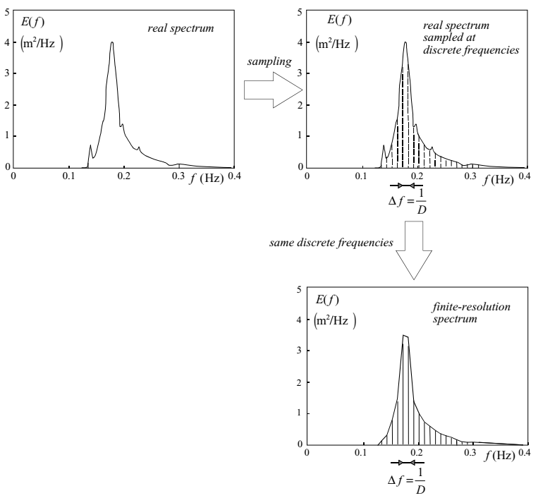

Figure 2.6: The finite frequency resolution, due to the finite duration of the wave record, removes details from the spectrum.

(Resolution is actually defined as the frequency interval between independent estimates of the spectral density, which in more advanced spectral-analysis techniques may differ slightly from 1/D.) The frequency resolution can be improved only by taking a longer duration of the wave record. However, the wave records should also be stationary to give the spectrum any meaning. The actual duration is therefore always a compromise. On the one hand it should be sufficiently short that the assumption of a stationary situation is reasonable, on the other hand it should be sufficiently long that the frequency resolution is adequate. In addition, it should be long enough to allow one to obtain statistically reliable estimates (see

3b One wave record

The fact that usually only one wave record is available for the spectral analysis (at least for measurements at sea) means that the variance density must be estimated (at least initially) from just one amplitude, i.e., from $\frac{1}{2} a^{2}_{i}$, rather than from $E\{\frac{1}{2}\underline{a}^{2}_{i}\}$. This gives the so-called ‘raw’ estimate of E(f):

\[\begin{equation} E(f) \approx \frac{1}{\Delta f} E\{\frac{1}{2}\underline{a}^{2}\} \rightarrow \boxed{\frac{1}{\Delta f} (\frac{1}{2}\underline{a}^{2})} \text{ with resolution } \Delta f = \frac{1}{D} \end{equation}\]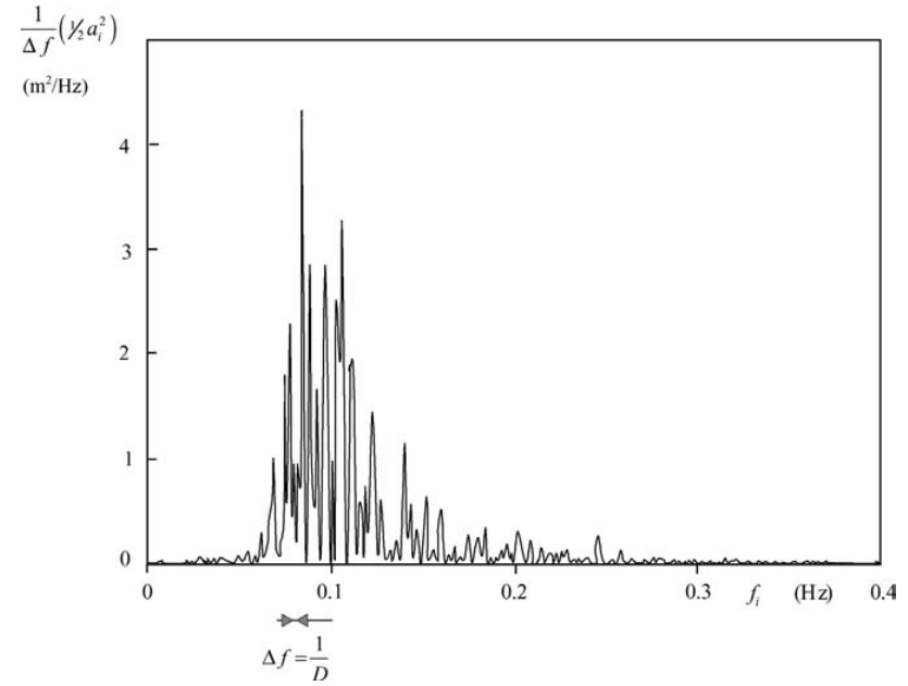

The raw spectrum looks ‘grassy’, because the variance density is estimated from only one amplitude per frequency (the error is of the order of 100%).

Figure 2.7: The raw spectrum looks ‘grassy’, because the variance density is estimated from only one amplitude per frequency (the error is of the order of 100%).

This raw estimate would be acceptable if the error (the difference between the expected value $E\{\frac{1}{2} \underline{a}^{2}_{i}\}$ and the computed value $\frac{1}{2} \underline{a}^{2}_{i}$) were relatively small, but that is not the case¹²; it is of the order of 100% (we can therefore not say $E(f) ≈ \frac{1}{2} \underline{a}^{2}_{i} /\Delta f )$. This large error is obvious from the rather ‘grassy’ look of the raw spectrum (see Fig. C.2). This poor reliability is unacceptable and it therefore needs to be improved (for the given wave record). This can be achieved only at the cost of something else.

There are several techniques to do this, but they all come at the expense of the spectral resolution. One of the simplest is to divide the time record into a number (p) of nonoverlapping segments, each with a duration $D^{∗} = D/p$. Each of these segments is then Fourier-analysed (as above) to obtain values of 1 2 a2 i with a resolution δf determined by the duration of the segment: $δf = 1/D^{∗} = 1/(D/p) = p \Delta f$ . The expectation $E\{\frac{1}{2} \underline{a}^{2}_{i}\}$ is then estimated as the average of these values (for each frequency separately; this is called the quasi-ensemble average, indicated with $\langle.\rangle$):

\[\begin{equation} E\{\frac{1}{2}\underline{a}^{2}\} \approx \langle\frac{1}{2} {a}^{2}\rangle \end{equation}\]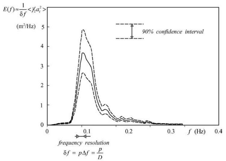

Figure 2.8: The (quasi-)ensemble-averaged spectrum of Fig. C.2 and its 90% confidence interval.

By this quasi-ensemble averaging, the error¹³ is reduced by a factor $\sqrt{p}$:

\[\begin{equation} \boxed{E(f) \approx \frac{1}{\delta f} \langle\frac{1}{2} a^{2}\rangle} \text{ with resolution } \boxed{\delta f = p \Delta f} \text{ and error } \boxed{\approx \frac{100%}{\sqrt{p}}} \end{equation}\]

Obviously, this improved reliability has come at the expense of the spectral resolution, which has been reduced by a factor of p. A compromise is therefore always required, in order to balance an acceptable spectral resolution against an acceptable reliability. A duration of 15−30 min and a value of p = 20–30 are typical for observations at sea. The corresponding frequency resolution is then δf ≈ 0.01−0.02 Hz and the error in the spectral densities is about 20%. The reliability may also be quantified with a confidence interval. This is the interval, within which the expected value is located with a certain probability, e.g., the 90% confidence interval (see Figs. C.3 and C.4).

3c The discrete wave record

In practice, the wave records are discretised by sampling the original signal of the wave sensor at a fixed time interval $\Delta t$. This interval is usually 0.5 s for wave observations at sea. A direct consequence of this discretisation is that the integrals in the above Fourier transforms are replaced with discrete sums, giving an error that is not so obvious. To illustrate this, consider a harmonic wave with frequency f1 that is sampled at a constant interval $\Delta t$

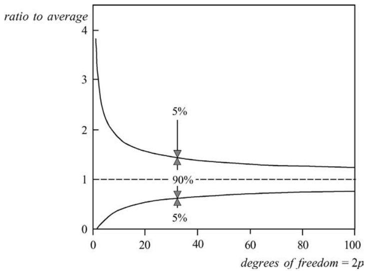
$The 90% confidence interval from the $\chi^{2}$-distribution.$

Figure 2.9: The 90% confidence interval from the $\chi^{2}$-distribution.

(the solid line, long wave in Fig. C.5). The only data available in the discrete record of this wave are the values at equidistant times (indicated with dots). However, it is entirely possible to have another harmonic wave (with frequency f2: the dashed line, short wave in Fig. C.5) with the same values at the same discrete moments in time (the same dots). A Fourier analysis, using these sampled elevations, therefore cannot distinguish the two wave components.

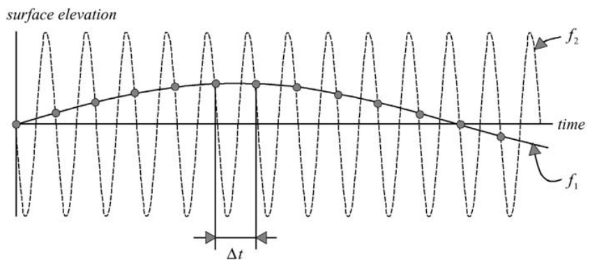
$Two harmonic waves with frequencies f1 and f2 that are given at discrete, constant time intervals $\Delta t = 1/( f1 + f2)$ are indistinguishable at these discrete times (as indicated by the dots).$

Figure 2.10: Two harmonic waves with frequencies f1 and f2 that are given at discrete, constant time intervals $\Delta t = 1/( f1 + f2)$ are indistinguishable at these discrete times (as indicated by the dots).

NOTE C2 The Nyquist frequency

The discretised wave record can be seen as the ‘true’ surface elevation multiplied by a delta series, i.e., a series of delta functions at interval $\Delta t$ (see the left-hand column in the figure below). Since multiplication in the time domain corresponds to convolution in the spectral domain, the wave spectrum should be convoluted with the spectrum of the delta series. Briefly stated, convolution is that each value of the one function is distributed in the shape of the other. Since the spectrum of the surface elevation is, strictly speaking, an even function (see Eq. 3.5.18) and the spectrum of a delta series is another delta series with interval $\Delta f = 1/\Delta t$, the result is a repetition of the (even) spectrum of the waves, with interval $f = 1/t $(see the right-hand column in the figure below). The effect is that the tails of the repeating spectra overlap, giving the impression that the frequencies $1/(2\Delta t), 1/\Delta t, 3/(2\Delta t), 2/\Delta t, 5/(2\Delta t)$, … etc. (multiples of the Nyquist frequency 1/(2t)) are mirror frequencies.

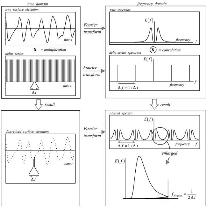
The consequence is that, in the spectral analysis, the energy density of the (high) frequency f2 is added to the energy density of the (low) frequency f1. It is as if the energy density of these high frequencies were mirrored around a frequency called the Nyquist frequency (or ‘mirror’ frequency; see Fig. C.6).

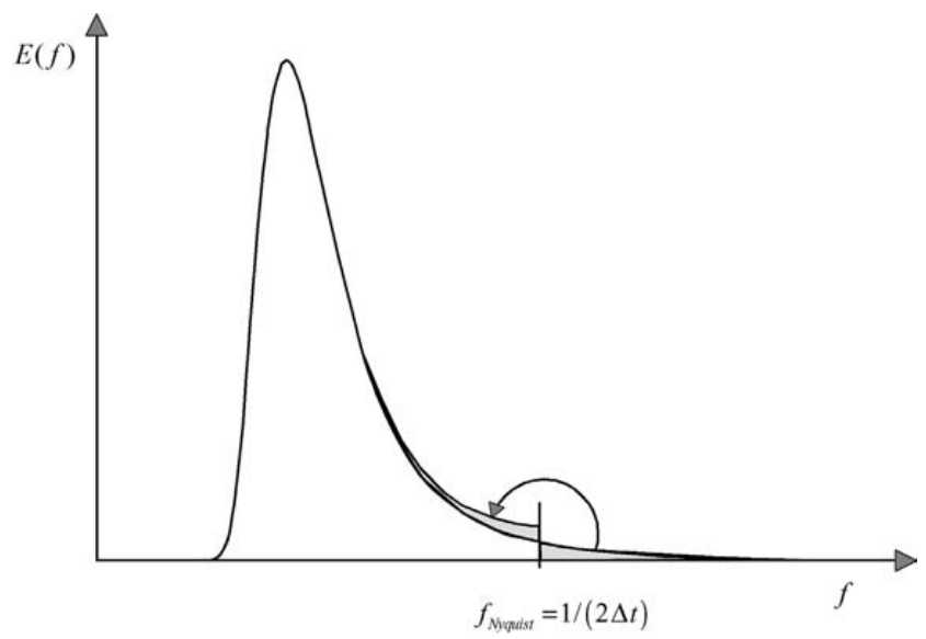
$Aliasing in the spectrum of a wave record with discrete time intervals $\Delta t$ is equivalent to mirroring the spectrum around the Nyquist frequency $f_{Nyquist} = 1/(2 \Delta t)$.$

Figure 2.11: Aliasing in the spectrum of a wave record with discrete time intervals $\Delta t$ is equivalent to mirroring the spectrum around the Nyquist frequency $f_{Nyquist} = 1/(2 \Delta t)$.

\[\begin{equation} \boxed{f_{Nyquist} = f_{N} = \frac{1}{2\Delta T}} \end{equation}\]

The high-frequency energy thus appears at other frequencies than those at which it should, in other words, under an ‘alias’. The phenomenon is therefore called ‘aliasing’. The aliasing phenomenon will always cause a relatively large error (about 100%) near the Nyquist frequency, but, with the rapidly decreasing energy densities in the tail of ocean wave spectra, it usually does not seriously affect the main part of the spectrum if the Nyquist frequency is chosen to be much higher than a characteristic frequency of the spectrum. The Nyquist frequency should therefore be chosen wisely, for instance more than four or five times the mean frequency (for measurements at sea, usually fNyquist = 1 Hz, corresponding to $\Delta t = 0.5 s$).

3d Instrument and processing noise

Measurements of the sea-surface elevation are always based on some physical characteristic of the water (surface) that is transformed by some instrument into numbers. These numbers do not exactly give the sea-surface elevation; they are always contaminated to some extent by the measurement technique, the instrument and the processing of the original signal. This difference is referred to as ‘observation noise’ or ‘instrument noise’. This subject is important for measuring ocean waves, but it is mentioned here only to make the reader aware of the problem.

An alternative type of analysis that is slowly gaining popularity as a supplement to the Fourier analysis is the wavelet analysis (e.g., Farge, 1992; Foufoula-Georgiou and Kumar, 1994; Mallat, 1998). It is essentially a variation on the Fourier analysis that is considered here.↩︎
Usually a Fourier series starts with i = 0 to include the mean value of the time series, but that has been taken to be zero here.↩︎
The harmonic x(t) = a cos(ωt + α) may be written (standard trigonometry) as x(t) = a[cos(ωt) cos α − sin(ωt) sin α], so that, if we write x(t) = A cos(ωt) + B sin(ωt), then A = a cos α and B = −a sin α. From this we find a2 = A2 + B2 and tan α = −B/A.↩︎
The amplitude $\underline{a}_{i}$ is Rayleigh distributed, so the distribution of $\frac{1}{2} a^{2}_{i}$ is an exponential distribution with a mean value $E\{\frac{1}{2} \underline{a}^{2}_{i}\}$ and a width equal to $E\{\frac{1}{2} \underline{a}^{2}_{i}\}$. In other words, the error associated with estimating $E\{\frac{1}{2} \underline{a}^{2}_{i}\}$ as $\frac{1}{2} \underline{a}^{2}_{i}$ is of the same order as the mean.↩︎
The distribution of this ensemble average $\langle\frac{1}{2} a^{2}\rangle$ is a $\chi^{2}$-distribution with 2p degrees of freedom.↩︎