Appendix A: Random variables
1 One random variable
1a Characterisation
The surface elevation in the presence of waves, at any one location and at any one moment in time, will be treated as a random variable (a variable the exact value of which cannot be predicted).
A random variable x is fully characterised by its probability density function p(x), which is defined such that the probability of x attaining a value between x and x + dx is given by (see Fig. A. 2.3).
\[\begin{equation} Pr\{x < \underline{x} \le x + dx\} = \int_{x}^{x+dx} p(x)dx \tag{A.1} \end{equation}\]
It follows that the probability of x being less than or equal to x (the probability of non-exceedance; see Fig. A.3) is
\[\begin{equation} Pr\{\underline{x} \le x\} = \int_{-\infty}^{x} p(x)dx = P(x) \end{equation}\]P(x) is called the (cumulative) distribution function of x. The above probability density function can be obtained as the derivative of this distribution function: p(x) = dP(x)/dx. Obviously, the value of a random variable is always less than infinity, so the probability that the value of x is less than ∞ is 1. This implies that the maximum value of the distribution function P(x) is 1 and that the surface area of a probability density function p(x) is always 1:
\[\begin{equation} Pr{\underline{x} \le \infty} = P(\infty) = \int_{-\infty}^{\infty} p(x)dx = 1 \end{equation}\]
Note that statisticians express probabilities in terms of fractions. The inverse of the distribution
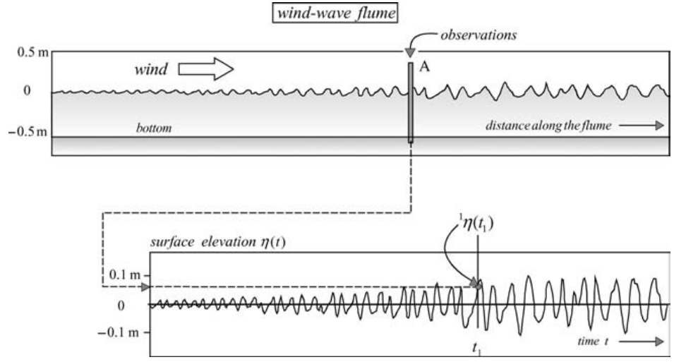
Figure 2.1: One value of the surface elevation 1 η(t1) at one location, one moment in time, in one experiment, in a wind-wave flume.
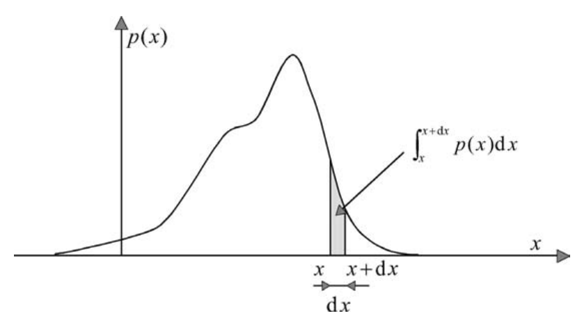
Figure 2.2: The probability density function p(x) of a random variable x.
%20distribution%20function%20P(x)%20of%20a%20random%20variable%20x%20(the%20probability%20of%20non-exceedance)%20_waves_book.png)
Figure 2.3: The (cumulative) distribution function P(x) of a random variable x (the probability of non-exceedance).
the function that gives the value of the random variable x for a given probability of non-exceedance, is written as x(P) = P−1(x) and is called the quantile function.
\[\begin{equation} \text{expected value of x} = E\{\underline{x}\} = \mu_{x} = \frac{m_{1}}{m_{0}} = \frac{\int_{-\infty}^{\infty} xp(x)dx}{\int_{-\infty}^{\infty} p(x)dx} \end{equation}\]
Since \(\int_{-\infty}^{\infty} p(x)dx = 1\), it follows that
\[\begin{equation} E\{\underline{x}\} = \mu_{x} = \int_{-\infty}^{\infty} xp(x)dx \end{equation}\]
This average may be interpreted as the location of the probability density function on the x-axis. The probability density function may be further characterised by increasingly higher-order moments. The second-, third- and fourth-order moments are thus used to define the width, skewness and kurtosis of the function respectively. For instance,
\[\begin{equation} \sigma_{x}^{2} = E\{(\underline{x} - \mu_{x})^{2}\} = \int_{-\infty}^{\infty} (x - \mu_{x})^{2} p(x)dx = E\{\underline{x}\} - \mu_{x})^{2} = m_{2} - m_{1}^{2} \end{equation}\]σ2 x is called the variance and σx the standard deviation of x, which represents the width of the probability density function.
The variance σ2 x of x can be seen as the average of the function f (x) = (x − µx ) 2. In general, the expected value of a function f (x) is defined as
\[\begin{equation} E\{f(x)\} = \int_{-\infty}^{\infty} f(x)p(x)dx \end{equation}\]1b Gaussian probability density function
Many processes in Nature behave in such a way that the well-known Gaussian probability density function applies:
\[\begin{equation} p(x) = \frac{1}{\sqrt{2 \pi \sigma_{x}}} \text{ exp } [-\frac{(x - \mu_{x})^{2}}{2 \sigma_{x}^{2}}] \end{equation}\]A theoretical explanation of this almost universal applicability is provided by the central limit theorem, which, simply formulated, says that the sum of a large number of independent random variables is Gaussian distributed.Many others may also apply, e.g., the Rayleigh, exponential and Weibull probability density functions.
1c Estimation
An average of a random variable x is often not determined from the probability density function p(x), but estimated from a set of sample values of x (called realisations, e.g., observations in an experiment).Such a set of sample values is called an ensemble, and the average is called an ensemble average, denoted as \(\langle.\rangle\). For instance,
\[\begin{equation} \begin{aligned} &\text{mean} = \mu_{x} \approx \langle \underline{x} \rangle = \frac{1}{N} \sum_{i=1}^{N} \underline{x}_{i} \end{aligned} \end{equation}\] \[\begin{equation} \begin{aligned} \text{variance} &= \sigma_{x}^{2} \approx \langle (\underline{x} - \langle \underline{x} \rangle)^{2} \rangle \\ &= \frac{1}{N} \sum_{i=1}^{N} (\underline{x}_{i} - \langle \underline{x} \rangle)^{2} = \frac{1}{N} \sum_{i=1}^{N} \langle \underline{x}_{i} \rangle^{2} - \langle \underline{x} \rangle^{2} \end{aligned} \end{equation}\]where N is the number of samples. Note that these are only estimates, which will always differ from the expected values. These differences are called (statistical) sampling errors.
2 Two random variables
2a Characterisation
A pair of random variables (x, y) is fully characterised by its joint probability density function: p(x, y).
\[\begin{equation} Pr\{x < \underline{x} \le x + dx \text{ and } y < \underline{y} \le y + dy \} = \int_{x}^{x+dx} \int_{y}^{y+dy} p(x, y)dxdy \end{equation}\]The two random variables may be unrelated to one another. They are then called independent. Alternatively, they may well be related. When they are linearly related they are said to be correlated. The degree of correlation (the degree to which the pairs of (x, y) cluster around a straight line) is quantified with the correlation coefficient γx,y , which is defined as the normalised covariance Cx,y of the two variables:
\[\begin{equation} \gamma_{x,y} = \frac{C_{x,y}}{(\sigma_{x}\sigma_{y})} \text{ with } -1 \le \gamma_{x,y} \le 1 \end{equation}\]where the covariance is the average product of \(\underline{x} \text{ and } \underline{y}\), each taken relative to its mean:
\[\begin{equation} C_{x,y} = E\{(\underline{x} - \mu_{x})(\underline{y} - \mu_{y})\} \end{equation}\]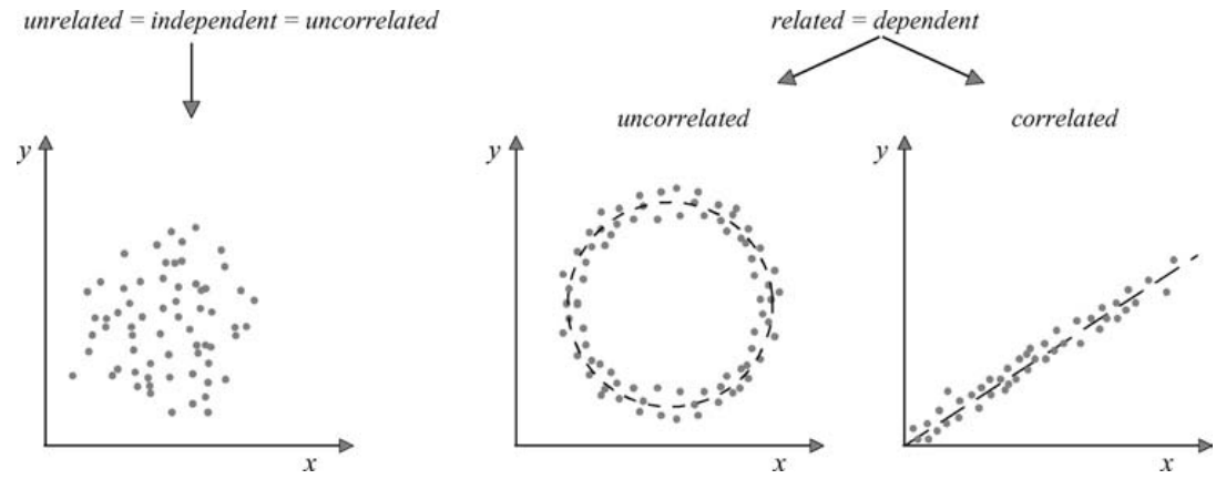
Figure 2.4: (In)dependent, (un)related and (un)correlated random variables.
3 Stochastic processes
3a Characterisation
Random variables may not only be dependent, related or correlated. They may also be ordered in some sense, i.e., the variables exist in some kind of sequence. This is a useful notion when (many) more than two variables are considered. Such an ordered set of random variables is called a stochastic process.
A stochastic process in one-dimension can readily be visualised with the wind-generated waves in the flume of Section 1a of this appendix. The measurement starts at t = 0 when the wind starts to blow over still water and the subsequent (very large) set of surface elevations η observed at location A is a function of time.
(Note that, in a time sequence x(ti), the random variable x at time t1 is another random variable than x at time t2, which is another random variable than x at time t3, etc.). One such experiment is one realisation of the stochastic process η(t1), η(t2), η(t3), . . ., η(ti), . . . .
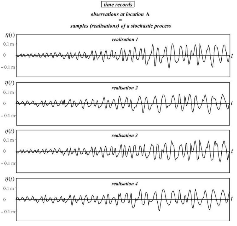
Figure 2.5: A set of four realisations of the surface elevation as a function of time, at location A, in the laboratory flume of Fig. A.1 (statistically identical experiments, but with the same wind speed etc.). The waves grow as time increases until some sort of equilibrium (in a statistical sense) is reached (i.e., stationarity).
Obviously, there are as many realisations of the stochastic process η(t1), η(t2), η(t3), . . ., η(ti), . . . as there are experiments (see Fig. A.5).
To characterise the surface elevations as a process, we need additionally, at that moment in time ti , all joint probability density functions, i.e., the joint probability p(η(ti), η(tj)) for all tj. There is an infinite number of moments in time ti , each requiring an infinite number of such functions, since there are infinitely many moments tj!
3b Stationary processes
If, after some time, the surface elevation at location A in the flume is constant in some statisticalsense (see Fig. A.5), then all statistical characteristics of the waves are independent of time and the process is said to be stationary (but the statistical characteristics may still depend on time intervals tj − ti). If only the averages and the variances of the variables are constant in time or space, the process is called weakly stationary or weakly homogeneous.
3c Gaussian processes
If all (joint) probability density functions of a process (stationary or not) are Gaussian, the process is called a Gaussian process. A Gaussian process is relatively simple to describe, since only the averages of each pair of variables and their covariance are required. Writing the variables of one such pair (see Eq. A.13) as x = x (t1) = x (t) and y = x(t2) = x(t + τ ), we may write the covariance as Cx,x = E{[x(t) − µx (t)] × [x(t + τ ) − µx (t + τ )]} = C(t, τ ). The covariance may therefore also be seen as a function of time t and time interval τ : the covariance function. Since the two variables are from the same process, C(t, τ ) is also called the auto-covariance function.
3d Stationary, Gaussian processes
A stationary, Gaussian process is even simpler to describe: only the mean and the covariances for one moment in time are required (because they are identical at all other times). The autocovariance is then (only) a function of the time interval τ and, if the average of the variable is taken to be zero (as usual for the surface elevation of waves), it can be written as
\[\begin{equation} C(\tau) = E\{(x(t) x(t + \tau)\} \end{equation}\]Note that the auto-covariance for τ = 0 is the variance of this process: \(E\{x^{2}(t)\} = C(0)\).
3e Ergodic processes
If averaging over time (or space) gives the same results as averaging over an ensemble of realisations, the process is said to be ergodic. The mean and variance of a zero-mean ergodic process can then be estimated as
\[\begin{equation} \mu_{x} \approx \langle \underline{x}(t_{i}) \rangle = \frac{1}{D} \int_{D} \underline{x}(t)dt \text{ (mean)} \end{equation}\] \[\begin{equation} \sigma_{x}^{2} \approx \langle [\underline{x}(t_{i})]^{2} \rangle = \frac{1}{D} \int_{D} [\underline{x}(t)]^{2}dt \text{ (variance) if } \mu_{x} = 0 \end{equation}\]and the auto-covariance as
\[\begin{equation} C(\tau) \approx \langle x(t)x(t + \tau) \rangle = \frac{1}{D} \int_{D} [\underline{x}(t) \underline{x}(t + \tau)]dt \text{ if } \mu_{x} = 0 \end{equation}\]where the brackets \(\langle . \rangle\) denote ensemble averaging and D is the length of the time interval (duration) over which the time average is taken. More generally, for the average of a function \(f[\underline{x}(t_{i})]\)
\[\begin{equation} \langle f[\underline{x}(t_{i})] \rangle = \frac{1}{D} \int_{D} f[\underline{x}(t)]dt \text{ for an ergodic process } \end{equation}\]It follows that such a process is stationary.8 The surface elevation of random, wind-generated waves under stationary conditions happens to be ergodic (in the linear approximation of these waves), so all averages needed to describe waves can be estimated as time-averages. This is fortunate because we would not be able to obtain an ensemble in Nature it would require Nature repeating, over and over again, identical conditions, in a statistical sense, at sea.
4 The sea-surface elevation
The surface elevation of wind-generated waves as a function of time is often treated as a Gaussian process. Measurements have shown this to be very reasonable (see Section 4.3), but there are also theoretical grounds: the surface elevation at any one moment in time ti can be seen as the sum of the elevations at that time of a large number of harmonic wave components that have been generated independently of each other (by a turbulent wind, possibly at very different locations) and that have travelled independently of each other across the sea surface (in the linear approximation of waves). The central limit theorem (see Section 1b of this appendix) shows that therefore the sea-surface elevation should be Gaussian distributed – but not always. Steep waves, or high waves in shallow water, do interact and are therefore not independent. Deviations from the Gaussian model do therefore occur at sea, particularly in the surf zone.
The reverse is not true: not all stationary stochastic processes are ergodic, for instance, switching on an electric circuit that produces an unpredictable but constant current (which may well be Gaussian distributed, i.e., the constant value is drawn from a Gaussian distribution every time the circuit is activated) gives a stationary, stochastic process (after all, the values are unpredictable and the statistical characteristics are constant in time). However, it is not an ergodic process because the time-average in each realisation is different from the time-average in another realisation, and is therefore (in general) not equal to the ensemble average.↩︎